From Lab to Live: Understanding Why Production Environments Erode Machine Learning Model Performance

Photo: Ecole polytechnique / Jérémy Barande, CC BY-SA 2.0, via Wikimedia Commons
At COSP10 Research Hub, we treat machine learning systems the way signal engineers treat transmission lines: the quality of the output depends not just on what was encoded at the source, but on what the channel does to the signal in transit. A model trained in a controlled environment is a signal encoded under ideal conditions. Production deployment is the channel — noisy, nonstationary, and rarely as well-behaved as the development environment suggested.
The gap between training-time performance and production-time behavior is one of the most persistent and consequential problems in applied machine learning. It is not a new observation — the research literature has documented it under various labels for over a decade — but it remains underaddressed in engineering practice. Teams celebrate validation accuracy, ship models, and then encounter a quieter, slower form of failure: gradual performance erosion that is difficult to detect, harder to diagnose, and expensive to remediate after the fact.
This article decodes the mechanisms behind that erosion and provides a structured framework for engineering teams to detect and respond to it systematically.
The Controlled Environment Illusion
Model development proceeds under conditions that are, by necessity, artificial. Training data is collected, cleaned, and partitioned. Feature engineering pipelines are designed against a snapshot of the data distribution. Hyperparameters are tuned against a held-out validation set drawn from the same underlying population. The entire optimization process is calibrated to perform well on data that resembles the training corpus.
This is not a flaw in methodology — it is an unavoidable structural property of supervised learning. The problem arises when the implicit assumption embedded in this process — that future production data will resemble historical training data — turns out to be wrong. And in practice, it almost always turns out to be wrong, to varying degrees, over varying timescales.
The divergence between the distribution of data seen during training and the distribution encountered in production is the root cause of the majority of post-deployment performance failures. Understanding its specific forms is the prerequisite for addressing it.
Distribution Shift: The Primary Decay Mechanism
Distribution shift is the general term for the mismatch between training and production data distributions. It manifests in several distinct subtypes, each with different diagnostic signatures and remediation strategies.
Covariate shift occurs when the marginal distribution of input features changes between training and deployment, while the conditional relationship between features and labels remains stable. A fraud detection model trained on transaction patterns from 2022 may encounter substantially different spending behaviors in 2025 — not because the underlying logic of fraud has changed, but because consumer behavior, merchant categories, and payment methods have evolved. The model's learned boundaries remain structurally valid; they are simply applied to inputs that no longer cluster the way the training data did.
Label shift presents a different problem: the prior probability of each class changes in production. A model trained on a dataset where fraudulent transactions represent 0.5% of samples may be deployed into a market segment where the base rate is 2.1%. Without recalibration, the model's confidence scores become systematically miscalibrated, producing either excessive false positives or missed detections depending on the decision threshold.
Concept drift is the most structurally challenging variant. Here, the underlying relationship between features and labels changes over time. This is common in natural language processing applications, where the semantic associations between words and sentiment shift with cultural context, and in financial modeling, where the predictive relationship between macroeconomic indicators and outcomes evolves with market regimes. No amount of additional training data from the original distribution will resolve concept drift; the model must be retrained on data that reflects the new relationship.
Feature Engineering Assumptions: The Silent Fragility Layer
Beneath distribution shift lies a more granular failure mode that engineering teams frequently overlook during development: the brittleness of feature engineering assumptions.
Feature pipelines encode implicit hypotheses about data structure. A pipeline that computes a rolling 30-day average assumes that 30 days of historical records will always be available for every inference request. A pipeline that one-hot encodes a categorical variable assumes the set of valid categories is closed and stable. A pipeline that normalizes a continuous variable against training-set statistics assumes those statistics remain representative in production.
Each of these assumptions can fail silently. When a production system encounters a new categorical value not present in the training vocabulary, many implementations default to a zero vector or an out-of-vocabulary token — and the model proceeds without any indication that its input representation has been degraded. When a data source upstream of the feature pipeline changes its schema, downstream features may be computed incorrectly without triggering any error condition visible to the model monitoring layer.
The result is a class of production failures that appear in model performance metrics but are invisible to infrastructure monitoring. The model is receiving degraded inputs and producing degraded outputs; the infrastructure stack reports all services as healthy.
Temporal Drift: The Slow Erosion
Distinct from abrupt distribution shift, temporal drift describes the gradual, continuous evolution of data characteristics over time. It is the most common form of production degradation for models deployed in consumer-facing applications and is the least likely to trigger alert thresholds set against short-term performance windows.
Consider a recommendation model deployed on a US streaming platform. At launch, the model's training data accurately reflects user preference patterns. Over six months, the user base grows, content libraries expand, cultural events shift viewing behaviors, and seasonal patterns introduce cyclical variation. No single week shows a dramatic performance drop. But the cumulative drift over the deployment period can reduce recommendation relevance by a measurable margin — one that becomes visible only in longitudinal A/B testing or cohort-level engagement analysis.
The engineering challenge with temporal drift is that standard monitoring approaches — tracking aggregate metrics like AUC or precision/recall on recent data — are often too coarse to detect slow degradation before it becomes user-impacting. More sensitive detection requires monitoring the statistical properties of input feature distributions directly, using techniques such as Population Stability Index (PSI) calculations or Kolmogorov-Smirnov tests applied to rolling windows of production data.
A Detection and Mitigation Framework for ML Engineering Teams
Addressing production performance decay requires both monitoring infrastructure and organizational process. The following framework reflects current best practices for US-based ML engineering teams operating at production scale.
Instrument the input distribution, not just the output metrics. Model performance metrics are lagging indicators. By the time accuracy or F1 scores degrade to threshold levels, the underlying data shift has typically been present for days or weeks. Monitoring the statistical properties of input features — mean, variance, entropy, null rates, category frequency distributions — provides earlier warning signals.
Establish baseline distribution profiles at training time. Before deploying a model, compute and store summary statistics for every feature in the production pipeline. These baselines serve as the reference point for ongoing drift detection. Without them, production monitoring has no stable reference signal to compare against.
Implement shadow deployment pipelines for model candidates. Running a challenger model in parallel with a production model — receiving live traffic but not serving predictions to users — allows performance comparison under real production conditions before any user-facing risk is incurred. This practice is standard at mature ML organizations and should be treated as a deployment prerequisite rather than an optional enhancement.
Define retraining triggers based on drift metrics, not calendar schedules. Scheduled retraining (e.g., monthly model refreshes) is a proxy for the actual goal: keeping the model calibrated to the current data distribution. Drift-triggered retraining, initiated when feature distribution metrics exceed predefined thresholds, is more responsive and less likely to either over-train on stable distributions or under-respond to rapid shifts.
Treat feature pipeline versioning as a first-class engineering concern. Feature transformation logic should be versioned, tested, and deployed with the same rigor applied to model weights. Schema changes in upstream data sources should trigger automated compatibility checks against the feature pipeline specification. Silent feature degradation is preventable with adequate pipeline instrumentation.
Conclusion: Closing the Signal Loop Between Training and Production
The performance gap between a model's development environment and its production behavior is not a failure of machine learning methodology — it is an expected property of deploying statistical systems into nonstationary environments. The engineering discipline required to manage this gap is distinct from the discipline required to build accurate models in the first place, and it demands its own infrastructure, tooling, and organizational attention.
For ML engineering teams, the goal is to close the signal loop: to build monitoring systems sensitive enough to detect early-stage drift, diagnostic frameworks capable of identifying its root cause, and retraining pipelines responsive enough to restore calibration before degradation becomes user-visible. The models that perform well in production over sustained deployment periods are not necessarily the ones with the highest validation accuracy at launch — they are the ones supported by the most rigorous production observability infrastructure.